This article explains how to include covariates in your Hierarchical Bayes (HB) MaxDiff analysis to improve its accuracy. Advances in computing have made it simple to include complex respondent-specific covariates in HB MaxDiff models. A few reasons why we may want to do this in practice:
- A standard model which assumes each respondent's part-worth (utility) is drawn from the same normal distribution may be too simplistic. Information drawn from additional covariates may improve the estimates of the part-worths. This is likely to be the case for surveys in which there were fewer questions and therefore less information.
- Additionally, when respondents are segmented, we may be worried that the estimates for one segment are biased. Another concern is that HB may shrink the segment means overly close to each other. This is especially problematic if sample sizes vary greatly between segments.
In this example, we'll take a MaxDiff analysis that does not use covariates:
and include them to produce a more accurate model:
Requirements
- Familiarity with MaxDiff anlaysis, check out our Introduction to MaxDiff article.
- A Hierarchical Bayes MaxDiff analysis output, see How to Use Hierarchical Bayes for MaxDiff for more info on what is required to prepare this. The raw data used in the example below is located here and design file here: http://docs.displayr.com/images/8/88/President_Experimental_Design.csv Our data set asked 315 Americans ten questions about the attributes they look for in a U.S. president. Each question asked the respondents to pick their most and least important attributes from a set of five. MDVersion is the Version variable. MDmost and MDleast are the best and worst variables.
Method
Step 1: Opening the document
- Create a new Q project and call it Presidential MaxDiff.
- Download the raw data file located here.
- Select File > Data Sets > Add to Project > From File and select the data file that you just downloaded.
Step 2: Fitting the MaxDiff model
- Select Create > Marketing > MaxDiff > Hierarchical Bayes
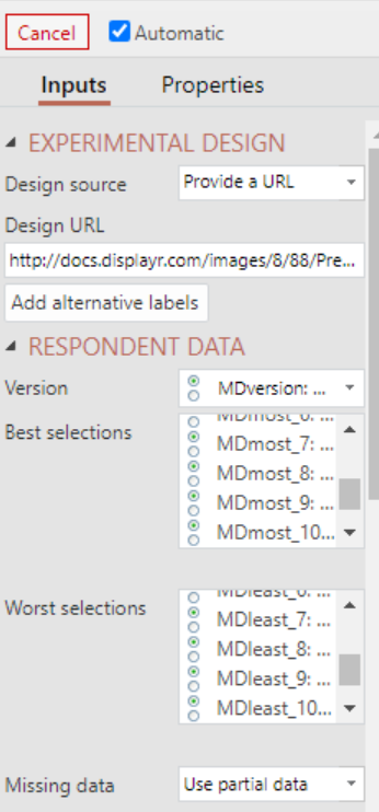
- In the Inputs tab:
- Design location: Provide a URL
- Design URL: http://docs.displayr.com/images/8/88/President_Experimental_Design.csv (MaxDiff is an experimental method, and its analysis requires both raw data and the experimental design).
- Version: MDversion: MaxDiff Version [MDversion]
- Best selections: Type mdmost and select the 10 variables. Make sure you select them in the correct order.
- Worst selections: Select the 10 mdleast variables.
- Add Alternative labels (if necessary): Add these alternatives in the spreadsheet that opens: Decent/ethical, Plain-speaking, Healthy, Successful in business, Good in a crisis, Experienced in government, Concerned for the welfare of minorities, Understands economics, Concerned about global warming, Concerned about poverty, Has served in the military, Multilingual, Entertaining, Male, From a traditional American background, Christian
- Model > Covariates: select your covariate variable
- Click Calculate. This calculation is going to take about 10 minutes or so (it is doing a lot!). The current MaxDiff output will be updated to show the results adjusted by the covariates.
- Check that the algorithm used has both converged to and adequately sampled from the posterior distribution, see this post for a detailed overview.
You can see that the In-sample accuracy of the model using the covariates increased slightly from 86.5% to 88.2% vs an increased computational time of about 5 minutes (because adding in the covariates makes the model more complex).
Technical Notes
In the usual HB model, we model the part-worths for the ith respondent as βi~ N(μ, ∑). Note that the mean and covariance parameters μ and ∑ do not depend on i and are the same for each respondent in the population. The simplest way to include respondent-specific covariates in the model is to modify μ to be dependent on the respondent's covariates.
We do this by modifying the model for the part-worths to βi~N(Θxi, ∑) where xiis a vector of known covariate values for the ith respondent and Θ is a matrix of unknown regression coefficients. Each row of Θ is given a multivariate normal prior. The covariance matrix, ∑, is re-expressed into two parts: a correlation matrix and a vector of scales, and each part receives its own prior distribution.
Displayr uses the No-U-Turn sampler from stan - the state-of-the-art software for fitting Bayesian models. This package allows us to quickly and efficiently estimate our model without having to worry about selecting the tuning parameters that are frequently a major hassle in Bayesian computation and machine learning. We fit the models using 1000 iterations and eight Markov chains. The package also provides a number of features for visualizing the results and diagnosing any issues with the model fit.
Next
How to Use Hierarchical Bayes for MaxDiff in Q
Case Study: Advanced Analysis of Experimental Data (MaxDiff)
Machine Learning - Diagnostic - Prediction-Accuracy Table