Introduction
Correspondence analysis is often used to visualize a table of data. The goal is to represent as much information as possible, as accurately as possible. However, there may be circumstances when we are interested in a specific row of the table (usually a brand). Such a point may not be represented well in the standard scatterplot output. In this post we explain a new technique developed by Q for rotating the results of correspondence analysis to focus on a specific point.
Correspondence analysis outputs consist of coordinates (usually plotted on a scatterplot) that explain the most variation across all of the brands. When we are interested in a specific brand, it can be useful to use focused rotation, described below. This is a novel technique that we have developed, described in the paper A brand’s eye view of correspondence analysis published in the International Journal of Market Research.
The data we are using in this article describes the characteristics that people associate with cars. The input table below is labelled by 14 car brands along the rows. The columns are labelled by characteristics. Each cell indicates the strength of association between a characteristic and a car.
Requirements
A table with multiple rows and columns containing data that are all on the same scale. This includes crosstabs showing counts, percentages, or averages, grids of data created from binary variables, and even raw numeric data.
Method
Initial Analysis
- From the toolbar, select Create > Dimension Reduction > Correspondence Analysis of a Table.
The results are as follows:

The data is plotted with normalization of principal coordinates. This means that we can compare distances between column labels and distances between row labels, but not the distance between a row and a column label. See this post for a more in-depth discussion about normalization and interpretation of correspondence analysis.
The dimensions output by correspondence analysis are in decreasing order of variance explained. This means that later dimensions explain smaller portions of the variance. The chart shows only the first two dimensions, which for this example, capture only 53.4% of the variance. So the hidden dimensions contain a reasonable amount of information. Importantly, from the plot alone we cannot tell how much information about any given point (brand) is retained.
Our first car
As an example, Mini Cooper is relatively close to the origin. This could be because it is poorly represented by the two plotted dimensions. Or it could genuinely be the case that Mini Cooper is close to the origin in all dimensions.
If we were performing this analysis to find the relationship of Mini Cooper to the other cars and characteristics, we could not draw any strong conclusions from this plot. The best we could say is that in the first two dimensions alone, there is little to discriminate it.
Quality of the map
We can create a table showing how much variance is represented in each dimension by doing the following:
- From the toolbar, select Create > Dimension Reduction > Diagnostic > Quality.
The resulting table (below) shows the variance in the first two dimensions before the row label of each car. Since Mini Cooper has only 16%, we can now say that the plot above hides much of the information for this brand.
Making a sharp turn
In order to find out more about the Mini, we rotate the results so that all of its variance is in the first dimension. This means that there is no longer any hidden information about this point. We shift the focus of the output onto Mini Cooper.
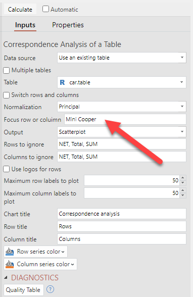
In Q, this is done by entering Mini Cooper in the box labeled Focus row or column. The effect of the rotation is shown below.
- In the Object Inpsector, type Mini Cooper in the Focus row or column box.

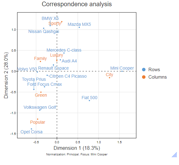
The results are as follows:

In this case, correspondence analysis produces embeddings in 5 dimensional space. If you find this difficult to visualize, join the club. What matters here is that there is no longer any hidden information about Mini Cooper. We can now see that it is more related to Fiat 500 than the other cars. This makes intuitive sense, as they are both small cars. We have gained insight by focusing on what differentiates Mini Cooper from the other cars.
However, note that the chart as a whole explains 46.3% of the variance in contrast to 53.4% in the first chart. The price we pay for the rotation is that the first two dimensions no longer contain as much variance as possible about all of the data. It is no longer the best general representation of all the points.
Buying a new car
As another example, let’s rotate to focus on the VW Golf. Notice how the plot below is very similar to the original, except rotated on the page.
- In the Object Inpsector, type Volkswagen Golf in the Focus row or column box.
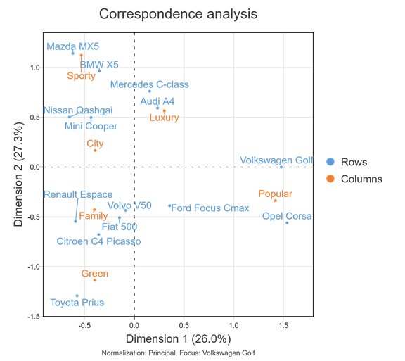
The results are as follows:

This rotation is easier to visualize. We have turned the page clockwise by about 135 degrees and the relationship between VW Golf and the other cars has been closely maintained. The total variance explained has dropped by only 0.1% from the original plot. All of this tells us that VW Golf was well represented originally. This confirms the 99% variance in the first two dimensions from the quality table above.
NEXT
How to Do Traditional Correspondence Analysis
How to Do a Multiple Correspondence Analysis
How to Create 3D Correspondence Analysis Plots in Q
How to Customize Bubble Charts for Correspondence Analysis in Q
How to Do a Correspondence Analysis of a Square Table
How to Add Images to a Correspondence Analysis Map in Q